Keeping Time and Energy in Closed Systems

The world is quantum, and we are part of the world. We should be able to make sense of observers inside of quantum systems; for instance, it might turn out that the universe is a closed system with us inside of it. Here I’ll try to puzzle through some confusing but elementary questions that arise. Although elementary, by the end we’ll find ourselves in a position to appreciate some recent advances quantum gravity. There’s also a bunch of references at the end if you want to know all the details.

The whole universe is too difficult, so let’s imagine ourselves in a smaller box, where time-evolution is described by some Hamiltonian acting on a Hilbert space. I will suppose that observers and measurement can be analyzed via unitary evolution plus decoherence, and being a closed system means that we consider only pure states of the system. Here’s a simple question: is total energy conserved?
Clearly, and uncontroversially, it is conserved on average, or in other words when summing all branches of a measurement. Just as clearly, it is not conserved in individual measurement outcomes: A superposition of states with very different energies can be collapsed even by even a very low-energy interaction (in Energy Non-Conservation in Quantum Mechanics, the authors give the example of a superposition between a bowling ball at rest and in motion being collapsed by the scattering of a single photon).

But the story does not end there. For instance, a question by Rochelle: If we repeatedly measure a subsystem in alternating bases, (only) one of them aligned with the energy basis, can the overall state then in principle gain energy unboundedly, even if such outcomes are very unlikely? Certainly it cannot lose energy indefinitely, because this would put total energy below zero after some finite time! This already tells us that we cannot ignore the step of ‘preparing the energy superposition’ in the algorithm.
It is actually easy to see that, at least if the energy distribution of the initial state is bounded above, no such loop can gain energy indefinitely. (By energy distribution I mean the classical probability distribution of total energy resulting from the Born rule $p_{\psi}(E)= \mid\mid \hat{p}_{E}|\psi\rangle\mid\mid^2$). At least within the realm of validity of Born rule measurements, meaning as long as decoherence is close to exact, the post-measurement state can be treated as a probabilistic mixture of its branches—and this being true is what makes it useful to speak of ‘measurement’ at all. In other words the energy distribution of the post-measurement state is a classical mixture distribution of the respective distributions of the branches. But since energy is preserved overall, this mixture distribution must be identical to the pre-measurement distribution of energy. In particular, ideal measurement cannot enlarge the support of the energy distribution in any branch—so there must be a limit to the possible energy gain even in individual branches.

We are faced with a curious consequence: to say that any measurement exhibits the initial energy distribution as a mixture of the possible post-measurement distributions is identical to saying that all changes in energy distribution are compatible with an interpretation as a classical knowledge update about total energy. In such a situation we’d usually say that total energy is subject to superselection. But here this conclusion would seem strange, since the system apparently cannot actually be in an energy eigenstate, as this would imply that there is no dynamics at all! Or does it? We’ll come back to this.
In the meantime, this does imply that it is impossible to actually demonstrate a violation of the claim that energy is exactly conserved in every outcome. The previously-mentioned example of a bowling ball in superposition between movement and rest is only possible to prepare when there is a sufficiently large pre-existing uncertainty in the energy which is transferred to the bowling ball in the preparation. We can then always say: look, the whole system always had this amount of energy, we just didn’t know it—and this assertion will be impossible to falsify.
Another mathematical consequence is that we must expect measures of energy spread, such as the variance or the entropy of the distribution, to decrease with every measurement, as we gain information. They may increase in individual outcomes, but in every measurement which does not leave the energy distribution entirely untouched they must decrease on average. So are we faced with a picture where all measurements tend to narrow the energy distribution, inexorably honing in on some precise value?

In Conservation Laws for Every Measurement Outcome Collins and Popescu demonstrate a loophole by which this may be avoided. The basic idea is this: when a subsystem is measured in some non-energy basis, the conventional formalism puts us into a product state like $|e\rangle|s\rangle$ after the measurement, where $|e\rangle$ is the environment and $|s\rangle$ is the system state which is not an energy eigenstate. In order to preserve energy exactly, the measurement procedure outlined in the paper instead allows some entanglement between environment and system. This technically puts the system into a mixed state so it might seem useless for describing genuine interference between energy eigenstates. But the insight is that the amount of entanglement necessary to preserve energy can be made incredibly small as long as $|e\rangle$ has a lot of energy uncertainty to begin with—so the difference to a product state will be undetectable.
In slightly more detail: say $|s\rangle$ is a coherent sum of two energy eigenstates $|s_{+}\rangle$ and $|s_{-}\rangle$. Then the ‘measurement’ puts us into a state $|e_{+}\rangle|s_{-}\rangle+|e_{-}\rangle|s_{+}\rangle$, where $|e_{+}\rangle$ and $|e_{-}\rangle$ are environment states with slightly shifted energies such that both summands have identical energy distributions. Now if the energy spread in the environment is extremely big to begin with, one sees that $|e_{+}\rangle$ and $|e_{-}\rangle$ can have very large overlap, so that this entangled state is essentially indistinguishable from $|e\rangle(|s_{-}\rangle+|s_{+}\rangle)=|e\rangle|s\rangle$. By increasing the energy spread in $|e\rangle$, we can in fact make the difference arbitrarily small while still preserving energy precisely.

This is a nice picture, which gives us a formalism of measurement in which conserved quantities are conserved exactly in every outcome. But does this describe real-world measurements? What about the other kind of measurement which genuinely does collapse a real energy spread in the state? Let’s return to our argument that total energy should be superselected for.
I’m going to argue that it is actually straightforwardly true that there is energy superselection, and that on the other hand there is a sense in which even an energy eigenstate can contain interesting dynamics. For comparison, let’s first consider the analogous situation for a different conserved quantity which is a bit more intuitive to think about.

Imagine that I am inside of a small closed-off lab floating in empty space, in which I can measure the locations and momenta of some particles. In this situation it is second nature to us—it is drilled into first-semester physics students—that I can only measure with respect to “the lab frame”, while judgements about the lab’s absolute speed are meaningless. Somewhat less attention is typically given to the fate of the reference frame concept once quantum mechanics comes into play. Naively one might think that once I measure the location of one of my test particles in the lab, the lab itself must be localized in space. After all, the lab is where the particle is.
This is wrong: measuring the particle still means measuring its position in the lab frame, meaning that there is a relational observable—a correlation—“position of particle relative to lab” onto whose eigenstate we project. To an outside observer, my whole lab might be delocalized in a state of exact momentum even while this relational observable still has a precise value. On the other hand, to me such an outside observer would in turn appear delocalized. One can switch between these reference frames: localized observer, localized lab. This, informally, is the concept of quantum reference frames, first introduced (using exactly this example, and then a more complicated one involving electric charge) by Susskind and Aharonov.

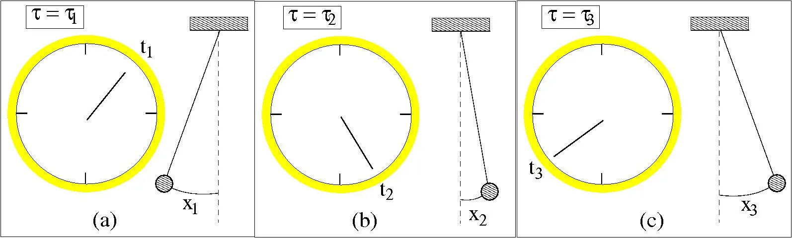
Now we return to energy. Everything works exactly the same, although this might not be immediately apparent. A reference frame for energy is called a clock, because that’s what it is. Usually in quantum mechanics we assume a formalism in which there is some true time variable $t$: this is equvialent to assuming the reference frame of some absolute ideal clock. An ideal clock can’t interact with the system itself and its existence makes no difference to us system-dwellers.
Now in the reference frame of an ideal clock (which is to say, in textbook QM), our analysis of an ever-narrowing energy spread was correct. But it means in turn that we ourselves become less localized in ideal time with each measurement. On the other hand, in our reference frame, defined by the physical clocks we actually have access to, the energy-conserving picture by Collins and Popescu prevails—if it didn’t, we’d become delocalized in time with respect to those clocks as well, which we don’t as long as we measure them occasionally. So to the extent that we believe in the accuracy of our clocks we should also believe in exact energy conservation, and if we don’t believe in our clocks we can’t make sense of energy in any case! And the residual entanglement in the Collins-Popescu picture can be directly seen as stabilizing our clocks.

I promised to show that even an energy eigenstate (and now we must add: with respect to ideal time) can contain nontrivial dynamics. This is what happens when delocalization in time is taken to its most extreme. We can be a bit more explicit (I’ve mostly been doing without formulas in this post, but see also the references at the end). What we do is we add an ideal clock to our system. Our clock’s Hilbert space is $L^{2}(\mathbb{R})$, which has a Hamiltonian such that at time $t$ it is in an eigenstate of the position operator along $\mathbb{R}$ (so the state is a $\delta$-distribution moving along the line with unit speed). We tensor the system with this Hilbert space, adding no interaction between system and clock. If we start out at time $t=0$ with some initial condition $|\psi\rangle$ of our system, then system and clock are in a product state and remain so at every precise instant of time.
Now to delocalise we group-average, that is we consider the state $\Psi =\int |\psi(t)\rangle|t\rangle dt$, where $|t\rangle$ denotes clock eigenstates. This is the average over evolution of the initial state, so the projection of combined clock+system to a state of $0$ total energy. Ideally we’d like to perform the integral over all time, for which we’d have to compactify time on a circle. But imposing some far-off integration boundaries is also not disastrous, we merely incur some arbitrarily small inacurracy.
The state $\Psi$ is static but contains the full time-evolution: $\psi(t)$ can be recovered by conditioning on a definite clock state: by projecting $\Psi$ onto the subspace $\mathcal H_{S}\otimes|t\rangle$. This is what’s known as the Page-Wootters mechanism. The relational observables which make physical sense are the correlations between the clock and the system. Representation-theoretically, the group-averaging operation is simply the norm map, and all we’ve done is observed that this gives us an isomorphism between orbits and invariant states.
Of course, we were only able to achieve this by adding an ideal clock, which is not realistic. A more physical scenario would have the clock be part of the system, which complicates things. For one, ideal clocks have unbounded-below energy spectrum across which the clock states are spread out. If we restrict the energy to be positive, we don’t get perfect $\delta$-localized clock states; the best we can do is the “Feynman kernel” ${i \over 2\pi(t+i \epsilon)}={1 \over 2}\delta(t)+\mathrm{p.v.\ } {i \over 2\pi t}$!

Quantum Gravity

All this is surprisingly relevant to quantum gravity. As Susskind puts it:

In classical general relativity without quantum mechanics a reference frame can be arbitrarily light so that it doesn’t gravitate and disturb the system. In quantum mechanics without gravity a reference frame can be arbitrarily heavy so that it doesn’t fluctuate. But in a world with both gravity and quantum mechanics, quantum reference frames will inevitably gravitate, fluctuate, and become entangled with the rest of the system. We cannot ignore them.

The Problem of Time in quantum gravity is this: for a time-reparametrization-invariant theory like general relativity, the Hamiltonian is constrained such that it vanishes on all trajectories—the equations of motion say $H=0$. Classically, this is not an obstruction to having a Hamiltonian formulation of GR, since we can still have nonvanishing derivatives of $H$ in “off-shell” directions and these furnish our Poisson brackets. But if we try to quantize this, the fact that $H|\psi\rangle=0$ means we have no notion of time-evolution. (This is the Wheeler-deWitt equation.)
But we know how to deal with this now! We’ve learned that such a state can contain dynamics. One only has to couch all observations as relative to the state of some clock subsystem. Clocks are all around us: the rotation of the earth around the sun is a clock, the cosmological scale factor, the rotation of galaxies and so on.
Actually, this is all very similar to how things already work classically: I think we should roughly think of states satisfying the Wheeler-deWitt constraint as “block universe states” containing a whole spacetime (or multiple branches of universes, etc). Classically also, all of the observable physics is contained in what the constraint $H=0$ says about clocks and rulers &c, and their joint states. This image is from the wikipedia article on Hamiltonian constraints and is not a priori about quantum mechanics, but you can see that the idea is the same:

There is a difficult question of how to actually identify clocks. This of course depends on what one takes as given. If one only starts with an abstract Hilbert space and a vector in it, up to isomorphism, one is clearly out of luck. We have to somehow, even if only approximately, be able to cut out a spatially localized subsystem containing a clock.
It’s conceivable that this is possible. It has been observed that in a quantifiable sense almost all Hamiltonians which are local with respect to some basis are local with respect to only one basis. Even when there is more than one local basis, there is again generically not a large amount of options. Which is to say that given an operator with real positive eigenvalues it is a sensible question to ask “is there a local basis, and if so how does time-evolution of the state look like with respect to the given operator”. In the old picture of time-evolution with an ideal clock, this allowed a perspective (“Mad Dog Everettianism”) in which one supposes only a state and its time-evolution (or equivalently, the Hamiltonian, even just as a list of eigenvalues) to be fundamentally real, and all else emergent. Now we know that this was equivalent to taking as given an ideal clock, where finding a clock is the very problem we want to solve. Nevertheless, one might hope that the Wheeler-deWitt constraint operator replacing the Hamiltonian contains enough information somehow, but I don’t know what the status of the research is there.
An intuition I have in this context is that in ordinary QM, the act of diagonalizing the Hamiltonian, producing a base-change matrices between local and energy bases, is what contains all of the physics. Give me an oracle which can perform these transformations efficiently, and I can compute any time-evolution efficiently, including “what will the state of this (approximate) turing machine with NP-hard program be 5000 years in the future”. Such a transformation matrix is then in effect a precomputed lookup-table for the dynamics. My feeling is that a similar role should be played by the Wheeler-DeWitt constraint operator: there should be something in the theory which gives this operator meaning, requiring maybe the existence of a larger Hilbert space of unconstrained states. (In contrast holography as far as I can tell only gives a dual description of the kernel).

But this is all old news. Here’s something new: Although we don’t know how to find clocks or reference frames from just a state, putting them in by hand is very useful, as exploited by the all-star CLPW paper which explicitly adds a worldline with a quantum reference frame (here called an observer) to the closed system of de Sitter spacetime with weak gravity. The reference frame is a non-ideal clock with energy bounded below and the headline result is that one obtains in this manner a type $II_{1}$ algebra of observables accessible to the observer. Although de Sitter space is a closed system, this algebra only describes part of it—the static patch of the observer—so like the algebras of QFT it has only mixed states. Unlike local QFT algebras however, “Type $II_{1}$” means in short: states on this algebra have a notion of trace and (von Neumann) entropy; and there is a state of maximal entropy, which describes empty de Sitter space from the perspective of the observer. This is what one expects classically if one takes entropy to mean generalized entropy, so ordinary entropy plus horizon area. (A somewhat bizarre but true statement in this framework is then that empty de Sitter space is a state of infinite temperature).
What prevents local QFT algebras from enjoying similar properties? Part of it is a UV divergence in the entaglement across the boundary of the described region. It’s interesting that describing the system in relation to a clock makes this go away. My tentative interpretation of this is that although in QFT there are a priori arbitrarily small fluctuations of the field which when cut off at a boundary produce the divergent entropy, these basically wash out to an observer even slightly smeared in time.

Using clocks as reference frames is clearly useful, but it’s a bit ham-fisted. One suspects that a fuller description would require using reference frames not just for time translation but for the whole gauge symmetry of GR. I think at present it’s not very clear how to do this, though. In general it is clear what we must condition on: ideally, everything that we can observe. It is less clear, I think, what the analogue of the time-averaged state should be. One proposal is the Hartle-Hawking no-boundary state, conditioned on the presence of an observer. At some point it resembles the problem of choosing your priors in Bayesian inference.

Something else that occurs in quantum gravity, especially with positive cosmological constant, is that observers have a bound on their entropy. The usual measurement semantics of quantum mechanics (Born rule & projection measurements) apply to the limit of an observer with infinite Hilbert space, now fundamentally disallowed. An Everettian should not have any problem with this, since to them the Born rule is only an approximate thing in any case. A similar approach is taken in the paper Quantum mechanics and observers for gravity in a closed universe. They consider “quantum mechanics” to be a theory which includes the Born rule but which only makes sense relative to a specification of an observer who is treated classically; It is a theory which only applies “up to inaccuracies of order $e^{-S_{O}}$”, where $S_{O}$ is the observer entropy (the log of their Hilbert space dimension). To me this is perfectly compatible with Everettianism, but it seems the authors consider it a modern spin on the Copenhagen interpretation. Earlier I suggested that we might need to have theory with a larger Hilbert space than what holography or the constraint operator gives us—this paper implements something like that (even though the interpretation is a bit different).

That’s all I wanted to say, I think. I hope it was halfway coherent. If you made it to here, please let me know! And here’s a bunch of places to learn more:

References

• These two talks are very nice:
  • Relational Perspectives in Quantum Gravity: The Role of Quantum Reference Frames - Anne-Catherine de la Hamette
  • Quantum reference frames and local algebras - Kasia Rejzner
• Papers about quantum reference frames generally:
  • The Trinity of Relational Quantum Dynamics
  • Equivalence of approaches to relational quantum dynamics in relativistic settings explaining also a connection to Newton-Wigner localization probabilities
  • Relational Dynamics with Periodic Clocks
• To learn about the application to observers in de Sitter spacetime:
  • Susskind’s characteristically oracular POV: Observers and Observations in de Sitter Space - Leonard Susskind
  • Witten: Edward Witten - Algebras in Quantum Field Theory and Gravity
  • The paper: An Algebra of Observables for de Sitter Space
  • There are some papers translating this explicitly into quantum reference frame language:
    • Gravitational entropy is observer-dependent also examines the case of multiple observers and the emergence of a semiclassical limit
    • Crossed products and quantum reference frames: on the observer-dependence of gravitational entropy more in-depth companion paper to the previous
    • Quantum reference frames, measurement schemes and the type of local algebras in quantum field theory
• Some more talks and papers:
  • Harlow on quantum mechanics in a closed universe as a theory relative to an observer: HEP Seminar - Quantum mechanics and observers for gravity in a closed universe
  • The paper: Quantum mechanics and observers for gravity in a closed universe
  • Comments on the Hartle-Hawking state and observers - Ying Zhao—“I think actually Lenny [Susskind] has been advocating for years that for a theory of a closed universe all you have are just the correlation functions […] and all the physics is encoded in this collection of correlation functions. And I didn’t understand that until.. I understood it myself”
  • Absolute entropy and the observer’s no-boundary state

7 likes

+1

6 comments, sorted by newest first

collapse comment

Rochelle

4d ago

This is intetesting. I think I have to get into the quantum reference frame thing...

It's usually considered an unworkable pathology of Newton-Wigner localization that a boost can de-localize a state, i.e. that two different observers disagree whether I'm localized, but I wonder now if its okay...

Replies 1 Likes 1

collapse comment

Rochelle

4d ago

In particular, NW position observable is indexed to a choice of hypersurface, Σ. It is poincare covariant if poincare is permitted to act on this choice of Σ. However, you can be NW(Σ)-localized while simultaneously NW(Σ')-delocalized. This is the superluminal spreading of the wavepacket.

Replies 1 Likes 1

collapse comment

Rochelle

4d ago

I have wondered what to make of this Σ index. Is it a problem? Is it okay? What does it represent? What part of the physical situation tells us its value?

Now it smells like NW position is a relational observable...

Replies 1 Likes 1

collapse comment

Gregor

4d ago

:^)
you will want to look at this paper from the references then! arxiv.org/pdf/2007.00580

Replies 1 Likes 2

collapse comment

Michael Kinyon

4d ago

Btw, the Kuchař mentioned there happens to be my father-in-law.

*starts singing "It's a Small World, after all..."*

Replies 1 Likes 3

collapse comment

John C. Baez

4d ago

I've met Kuchař! A lively and amusing speaker.

Replies 0 Likes 1